
01 / THE QUESTION
Can structure do more of the work?
A component’s behaviour depends on both its material and the geometry inside it. Cellular structures introduce spaces and connected walls into a volume, creating another way to influence how that component responds to a load.
For my MSc project, I investigated thin-walled spinodoid structures made from polyether ether ketone (PEEK) reinforced with multi-walled carbon nanotubes (MWCNTs). I wanted to understand their mechanical and piezoresistive performance: how they deform under compression, and how their electrical resistance changes during that deformation.
I connected computational geometry with physical fabrication and testing. I compared two geometry parameter settings and two wall thicknesses, then examined the printed specimens’ dimensions, relative densities, stiffness and resistance measurements.
02 / UNDERSTANDING SPINODOIDS
A complex surface, made into a thin wall.
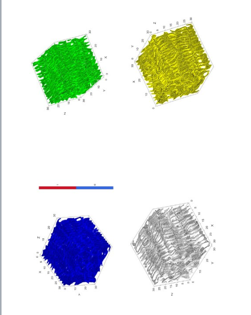
Spinodoids are cellular geometries inspired by the interconnected patterns associated with spinodal phase separation. Rather than drawing every opening individually, a mathematical field can describe a complex surface throughout a three-dimensional volume.
I used MATLAB and the GIBBON toolbox to generate the geometry. I extracted a surface and gave it a specified thickness to create a printable wall network. This let me vary the internal geometry while keeping the intended outer dimensions at 30 × 30 × 30 mm.
What do [90 0 0] and [45 0 0] mean?
I used these two settings to vary the directional character of the geometry. In my GIBBON code, they are the thetas parameters: conical half angles along x, y and z that control how the surface develops throughout the volume.
Another important quantity is relative density: the specimen’s bulk density divided by the reference solid material density. It describes how much material occupies the overall volume and helps interpret differences between the designed geometry and the printed part.
03 / FROM MODEL TO SPECIMEN
Design. Fabricate. Measure.
Generate the geometry
I generated and visualised the structure using GIBBON’s spinodoid function in MATLAB. I then extracted its isosurface, used
surf2solidto introduce a 0.40 mm or 0.48 mm wall, and exported the geometry as an STL file.Print and inspect
I fabricated the specimens using fused filament fabrication on an Apium P220 with MWCNT-reinforced PEEK. I measured each printed part’s mass and dimensions to evaluate its density and see how closely it matched the intended shape.
Record two responses together
I compressed the specimens in a universal testing machine, collecting force, displacement and time. I also connected a multimeter to the machine’s platens to record resistance and time during loading.
Compare the results
I converted force and displacement into stress and strain using the printed dimensions. I compared the elastic-region slopes and examined normalised resistance change during compression.
04 / THE EXPERIMENT
Four designs. Two specimen sets.
I designed four combinations of geometry and wall thickness, then measured and tested two printed sets. These were my intended dimensions; the actual printed dimensions varied.
| Model | Geometry setting [x y z] | Wall thickness | Nominal size |
|---|---|---|---|
| A | [90 0 0] | 0.40 mm | 30 × 30 × 30 mm |
| B | [90 0 0] | 0.48 mm | 30 × 30 × 30 mm |
| C | [45 0 0] | 0.40 mm | 30 × 30 × 30 mm |
| D | [45 0 0] | 0.48 mm | 30 × 30 × 30 mm |
Getting the structures to print successfully was part of the challenge. I worked through unsuccessful prints before comparing the test specimens. Model D in set 2 had a measured height of 25.63 mm, substantially below the intended 30 mm. That difference matters when comparing its response with the other specimens.
05 / WHAT THE TESTS SHOWED
Geometry matters. So does the printed part.
I calculated Young’s modulus from the elastic region of the stress–strain response. A higher value means a stiffer response in this comparison. The values below are my results for the individual specimens in each set.
| Model | Relative density Set 1 / Set 2 | Modulus Set 1 | Modulus Set 2 |
|---|---|---|---|
| A | 0.38 / 0.37 | 112.59 MPa | 115.67 MPa |
| B | 0.47 / 0.45 | 137.03 MPa | 122.70 MPa |
| C | 0.30 / 0.30 | 50.49 MPa | 40.00 MPa |
| D | 0.47 / 0.35 | 149.80 MPa | 88.15 MPa |
What I found
I found that, at 0.40 mm wall thickness, model A was stiffer than model C in both sets. Increasing the wall thickness from 0.40 mm to 0.48 mm also corresponded to higher measured modulus within each geometry setting in both sets.
The orientation comparison at 0.48 mm was mixed: model D exceeded B in set 1, while B exceeded D in set 2. D’s shorter printed height and lower relative density in set 2 complicate that comparison. I therefore considered the printed dimensions and densities alongside the stiffness results when comparing the two geometries.
The practical lesson
I learned to look beyond the nominal CAD design. Printed dimensions, density and fabrication consistency all mattered when interpreting the mechanical results. I also encountered testing errors and differences between the two sets’ stress–strain curves, which made the elastic region particularly useful for comparison.
06 / ELECTRICAL RESPONSE
Could the structure tell us how it is deforming?
I also investigated piezoresistive behaviour: a change in electrical resistance associated with mechanical strain. By recording resistance during compression, I could examine the electrical response alongside the mechanical measurements.
To compare that response with the starting measurement, I calculated normalised resistance change:
ΔR / R₀ = (R − R₀) / R₀
Here, R₀ is the initial resistance and R is the resistance at a later measurement. I plotted resistance and normalised resistance change over time, then took a closer look at the elastic region.
These measurements gave me a starting point for exploring how electrical response could indicate deformation and damage. My work focused on collecting and analysing that response. Building and validating a predictive model would be the next step.
07 / TAKEAWAYS
Connecting a digital idea to physical evidence.
Through this project, I brought geometry generation, additive manufacturing and experimental analysis into one workflow. I learned to consider geometry, material and manufacturing together: a promising model still needs to survive fabrication and produce interpretable test data.
I developed and tested thin-walled spinodoids while collecting mechanical and electrical measurements together. If I continued this work, I would test more repeat specimens, improve control over the printed geometry and test conditions, and independently validate any model relating resistance to deformation.
For me, that connection between design decisions and observed behaviour is the enduring value of the work: build something, measure what actually happens, and use the evidence to decide what to change next.
08 / MORE ABOUT MY WORK
Read more about my project.
I completed this project at the University of Glasgow as part of my MSc in Mechanical Engineering and submitted it on 19 August 2022 under the title Performance Evaluation of Additive Manufacturing Enabled Thin-Walled Spinodoid Structures.
I’m grateful to Professor Shanmugam Kumar and Lecturer Paul Prentice for their supervision, and to Alejandro Triay and Johannes Schneider for their support and guidance in the laboratory.